
Most discussions of large language models stay at the level of prompts, context windows and benchmark scores. That is fine for procurement, but it is not enough when you have to decide whether to fine-tune a model, how much GPU memory a deployment will need, or why a generation loop is slower than expected. Those answers sit one level down, in the arithmetic the model performs on every token.
So it is worth walking the path once, concretely. Take the prompt the cat, and follow what happens to the word cat from the moment it becomes an integer to the moment the model emits the next word. Classic dense decoder-only models repeat this sequence layer after layer; newer designs vary it, as in OpenAI’s gpt-oss (2025), which uses mixture-of-experts layers, and Alibaba’s Qwen3.5 (2026), which mixes Gated DeltaNet linear attention with standard attention; Alibaba’s Qwen3.8-Flash-Next (2026) pairs Gated DeltaNet with sparse attention instead.
Step one: the tokeniser decides what the model can see
Text has to become integers. A tokeniser holds a fixed vocabulary and maps each piece of text to an index in it. In a toy example, the and cat might become IDs 5 and 42. Real systems use subword schemes such as byte-pair encoding (Sennrich et al., 2016) or SentencePiece (Kudo and Richardson), which split rare or unusual words into several pieces, so the IDs for any given word depend entirely on the vocabulary the model was trained with.
This first step is less innocent than it looks. The tokeniser fixes the granularity at which the model perceives your domain. Product codes, chemical names, Greek or Arabic script, phone numbers and code identifiers can each fragment into many pieces under a vocabulary built mainly for English prose. That inflates sequence length, inflates cost per request, and spreads the signal for a single concept across several positions. If you are evaluating a base model for a specialised corpus, tokenising a representative sample and counting the pieces is one of the cheapest diagnostics available.
The residual stream: one vector per token
Each token ID indexes a row of a learned embedding matrix, producing a dense vector. On its own that vector carries no sense of order – cat in position one would be indistinguishable from cat in position five – so positional information is injected, classically by adding a position vector to the embedding, though modern models often encode position inside attention instead.
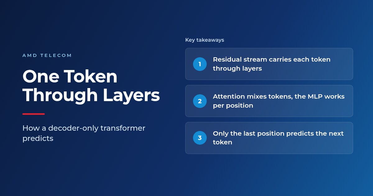
The result is the starting point of what is usefully called the residual stream: in classic designs a single vector per token that travels the whole depth of the network, although DeepSeek-V4 (2026) and Alibaba’s Qwen3.8-Flash-Next (2026) widen it into four parallel residual branches. Every block reads from this stream, computes something, and adds its result back. Nothing overwrites it. That additive structure is what lets gradients reach the earliest layers during training, and it is also why interpretability work can talk about individual components writing features into a shared channel. Practically, the residual stream is the thing you are reshaping when you fine-tune.
Attention: the only place tokens talk to each other
Inside a block, the stream is first normalised – in the pre-norm arrangement used by most current models, normalisation happens before the operation rather than after it – and then projected into queries, keys and values. These are split across attention heads. If the model dimension is 512 and there are 8 heads, each head works in 512 / 8 = 64 dimensions, so the heads cost roughly the same in total as one wide head while being free to specialise.
For our token, head zero forms a query from cat and compares it against the keys of every visible token. The comparison is a dot product divided by the square root of the head dimension (Vaswani et al., 2017); that scaling keeps the values in a range where the softmax does not saturate and stop producing useful gradients. The resulting weights are used to average the value vectors, the heads are concatenated, and a final output projection maps the result back to model dimension, where it is added to the residual stream.
Two properties matter commercially:
- Causal masking. cat may attend to
theand to itself, never to anything that comes later. This is what makes the model autoregressive, and what makes a decoder a generator rather than an encoder. - Cost. Attention is the only operation in which positions interact, and its compute grows quadratically with sequence length, while the rest of the block grows linearly. Long-context behaviour, and the memory it consumes, is decided here.
The MLP: per-token computation, most of the parameters
After attention comes the feed-forward block, again preceded by normalisation. It expands the vector to a wider inner dimension – four times the model dimension in the original transformer (Vaswani et al., 2017) – applies a non-linearity such as GELU (Hendrycks and Gimpel), contracts back to the original width, and adds the result to the residual stream.
Unlike attention, the MLP touches each position in isolation: no mixing, no awareness of neighbours. The usual division of labour is that attention moves information between positions while the MLP transforms what sits at each one. Because of the width expansion, this block holds the majority of a model’s parameters, which is why it is a main target of quantisation and sparsity work; the gating variants that replaced plain GELU in many recent models are covered in our article on SwiGLU and gated feed-forward blocks.
Attention, residual add, MLP, residual add – that is one layer. Stack it dozens of times and the representation of cat stops being a dictionary entry and becomes a prediction about what should follow it.
From final vector to next token
At the top of the stack, only the last position is used at inference time. Its vector is multiplied by the language-modelling head, an un-embedding matrix with one row per vocabulary entry, producing one score, or logit, for every possible next token. This matrix is large by itself: a 50,000-entry vocabulary and a model dimension of 4,096 gives 50,000 × 4,096 = 204.8 million parameters in that single layer.
Logits are then turned into a choice:
- Temperature rescales the logits before the softmax. Values below 1 sharpen the distribution towards the top candidates; values above 1 flatten it.
- Softmax converts the scaled scores into probabilities that sum to one.
- Sampling draws from that distribution, usually after restricting it with top-k or top-p truncation. This is the only step where randomness enters, and it is also the hook that structured-output methods use to force generations into a required format.
The sampled token is appended to the sequence and the whole process repeats. Note the asymmetry between the two regimes: during training the model predicts a next token at every position simultaneously, so a long document is one parallel pass; during generation it produces one token at a time, each pass depending on the last. To avoid recomputing the keys and values of earlier tokens at every step, they are cached – the memory consequences of that cache are the subject of our article on serving LLMs on your own GPUs.
What this means for organisations training and running their own models
Knowing the path a token takes changes how you read a specification and where you spend effort:
- Check the tokeniser against your data before anything else. If your domain fragments badly, downstream cost estimates will be wrong, and fine-tuning only partly compensates.
- Separate the two memory budgets. Weights are fixed; the key-value cache grows with batch size and sequence length. Capacity planning that ignores the second one under-provisions.
- Treat sampling settings as product configuration, not a detail. Temperature and truncation are per-request parameters and can be tuned for extraction and generation tasks independently, without retraining anything.
- Remember what training actually shapes. Fine-tuning adjusts what each block writes into the residual stream. The quality and consistency of the training data therefore usually matters more than the architectural choices available to you.
That last point is where most projects succeed or fail. AMD Telecom trains and fine-tunes deep-learning models and large language models on its own in-house GPUs, and uses BigParser, its in-house data collection platform, to turn web content and documents into structured training data.
If you are weighing up a model for your own domain, our AI Model Training and AI Model Development services cover the work from dataset construction through to a deployed model. Contact us to discuss what your data and your latency targets actually require.